Conceptual

1.

The best subset selection model for a given number of predictors will have an $RSS$ either smaller than or equal to the RSS of either stepwise selection model for the same number of predictors. This is because the metric determining model selection for a given count of predictors $k$ is minimization of RSS and best subset selection explores every possible combination of predictors $\binom{p}{k}$, whereas forward and backward stepwise selection only evaluate $(p-k)$ and $(k-1)$ models respectively.

Unable to say as there’s no suitable test error estimate taken into account when selecting a model for a particular number of predictors $k$. Generally speaking this is dependent on the extent to which the chosen learning method overfits the training data. Assuming overfit is not a huge problem then you would expect best subset selection to give the lowest test RSS, but the assumption cannot be tested without an appropriate validation strategy such as cross-validation in the first place.

i. True

ii. True

iii. False

iv. False

v. False

2.

iii. The lasso is simply least squares with the following additional constraint on the coefficient estimates.

$\sum\limits_{j=1}^p |\beta_j| \leq s$

The additional constraints means higher bias, if the increase in bias error is lower than the decrease in variance then prediction accuracy is improved.

iii. For the same reasons as above, but the constraint for ridge regression is:

$\sum\limits_{j=1}^p \beta_j^2 \leq s$

ii. Non linear methods are more flexible than least squares, hence variance will be greater. But if the underlying relationship is truly non-linear the decrease in bias will be greater and prediction accuracy will be increased.

3.

iv. Steadily decrease. When s = 0 all coefficients are constrained to 0 and training RSS will be maximized. When s is sufficiently large we obtain the ordinary least squares coefficient estimates and hence the lowest training RSS.

ii. Decrease initially, then increase. The OLS model will likely start overfitting the training data with a less strict constraint which lowers training RSS but doesn’t generalize to test RSS.

iii. As the constraint is relaxed more variance is introduced to the model.

iv. As the constraint is relaxed the squared bias of the model is reduced.

v. Remain constant, it’s called irreducible for a reason.

4.

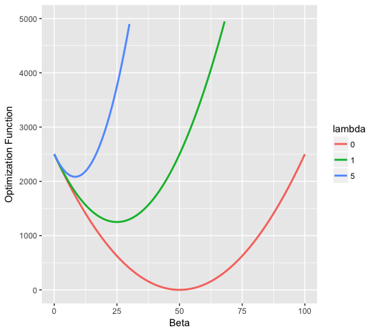
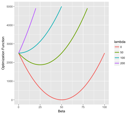
iii. When $\lambda$ is zero we have OLS which has the minimum training RSS by definition. As $\lambda$ is increased training RSS will decrease.

ii. We expect the ridge regression model to generalize better as it’s less prone to overfitting, hence test RSS will follow the usual characteristic U shape.

iv. As shrinkage parameter grows, flexibility decreases, hence variance decreases.

iii. As shrinkage parameter grows, flexibility decreases, hence bias increases.

v. IRREDUCIBLE.

5.

$\begin{align*} f(\beta_1, \beta_2) &= \sum\limits_{i=1}^n(y_i - \beta_0 - \sum\limits_{j=1}^p\beta_jx_{ij})^2 + \lambda\sum\limits_{j=1}^p\beta_j^2 \\ \end{align*}$

Under conditions:

$\beta_0 = 0 \\ x_{11} = x_{12} = x_1 \\ x_{21} = x_{22} = x_2 \\ y_1 + y_2 = 0 \\ x_{11} + x_{21} = 0 \\ x_{12} + x_{22} = 0$

Simplifies to:

$\begin{align*} f(\beta_1, \beta_2) &= 2(y_1 - x_1(\beta_1 + \beta_2))^2 + \lambda(\beta_1^2 + \beta_2^2) \end{align*}$

Partial derivatives:

$\begin{align*} \frac{\partial f(\beta_1, \beta_2)}{\partial \beta_1} &= 4(y_1 - x_1(\beta_1 + \beta_2))(-x_1) + 2\lambda\beta_1 \\ &= -2x_1(y_1 - x_1\beta_1 -x_1\beta_2) + \lambda\beta_1 \\ &= \beta_1(\lambda + 2x_1^2) + 2x_1^2\beta_2 - 2x_1y_1 \end{align*}$

and by clear symmetry,

$\begin{align*} \frac{\partial f(\beta_1, \beta_2)}{\partial \beta_2} &= \beta_2(\lambda + 2x_1^2) + 2x_1^2\beta_1 - 2x_1y_1 \end{align*}$

Set partial derivatives equal to zero.

$\begin{align*} \frac{\partial f(\beta_1, \beta_2)}{\partial \beta_1} &= 0 = \beta_1(\lambda + 2x_1^2) + 2x_1^2\beta_2 - 2x_1y_1 \\ \lambda\beta_1 &= 2x_1y_1 - 2x_1^2(\beta_1 + \beta_2) \end{align*}$ $\begin{align*} \frac{\partial f(\beta_1, \beta_2)}{\partial \beta_2} &= 0 = \beta_2(\lambda + 2x_1^2) + 2x_1^2\beta_1 - 2x_1y_1 \\ \lambda\beta_2 &= 2x_1y_1 - 2x_1^2(\beta_1 + \beta_2) = \lambda\beta_1 \end{align*}$

Hence $\beta_1 = \beta_2$.

We can borrow most of the math from part a as the penalty term is the only part that changes. Hence:

$\begin{align*} f(\beta_1, \beta_2) &= 2(y_1 - x_1(\beta_1 + \beta_2))^2 + \lambda(|\beta_1| + |\beta_2|) \end{align*}$

The lasso coefficients can’t be unique because taking the partial derivatives of the optimization function results in multiple cases as we’re taking the derivative of an absolute value. i.e.

For $\beta_1 > 0$,

$\begin{align*} \frac{\partial f(\beta_1, \beta_2)}{\partial \beta_1} &= 4(y_1 - x_1(\beta_1 + \beta_2))(-x_1) + \lambda\\ \end{align*}$

For $\beta_1 < 0$,

$\begin{align*} \frac{\partial f(\beta_1, \beta_2)}{\partial \beta_1} &= 4(y_1 - x_1(\beta_1 + \beta_2))(-x_1) - \lambda\\ \end{align*}$

And similarly for $\beta_2$, these solutions are found by setting each of these cases to 0.

6.

7.

Not entirely sure how to go about this.

Applied

8.

X = rnorm(100)
eps = rnorm(100)

b0 = 1
b1 = 1
b2 = 1
b3 = 1

Y = b0 + b1*X + b2*X^2 + b3*X^3 + eps

library(leaps)

df = data.frame(Y=Y, X=X)
rfit.full = regsubsets(Y ~ poly(X, 10), data=df, nvmax=10)
rfit.sum = summary(rfit.full)
rfit.sum

## Subset selection object
## Call: regsubsets.formula(Y ~ poly(X, 10), data = df, nvmax = 10)
## 10 Variables  (and intercept)
##               Forced in Forced out
## poly(X, 10)1      FALSE      FALSE
## poly(X, 10)2      FALSE      FALSE
## poly(X, 10)3      FALSE      FALSE
## poly(X, 10)4      FALSE      FALSE
## poly(X, 10)5      FALSE      FALSE
## poly(X, 10)6      FALSE      FALSE
## poly(X, 10)7      FALSE      FALSE
## poly(X, 10)8      FALSE      FALSE
## poly(X, 10)9      FALSE      FALSE
## poly(X, 10)10     FALSE      FALSE
## 1 subsets of each size up to 10
## Selection Algorithm: exhaustive
##           poly(X, 10)1 poly(X, 10)2 poly(X, 10)3 poly(X, 10)4 poly(X, 10)5
## 1  ( 1 )  "*"          " "          " "          " "          " "         
## 2  ( 1 )  "*"          " "          "*"          " "          " "         
## 3  ( 1 )  "*"          "*"          "*"          " "          " "         
## 4  ( 1 )  "*"          "*"          "*"          " "          "*"         
## 5  ( 1 )  "*"          "*"          "*"          " "          "*"         
## 6  ( 1 )  "*"          "*"          "*"          " "          "*"         
## 7  ( 1 )  "*"          "*"          "*"          "*"          "*"         
## 8  ( 1 )  "*"          "*"          "*"          "*"          "*"         
## 9  ( 1 )  "*"          "*"          "*"          "*"          "*"         
## 10  ( 1 ) "*"          "*"          "*"          "*"          "*"         
##           poly(X, 10)6 poly(X, 10)7 poly(X, 10)8 poly(X, 10)9
## 1  ( 1 )  " "          " "          " "          " "         
## 2  ( 1 )  " "          " "          " "          " "         
## 3  ( 1 )  " "          " "          " "          " "         
## 4  ( 1 )  " "          " "          " "          " "         
## 5  ( 1 )  "*"          " "          " "          " "         
## 6  ( 1 )  "*"          " "          " "          " "         
## 7  ( 1 )  "*"          " "          " "          " "         
## 8  ( 1 )  "*"          " "          " "          "*"         
## 9  ( 1 )  "*"          " "          "*"          "*"         
## 10  ( 1 ) "*"          "*"          "*"          "*"         
##           poly(X, 10)10
## 1  ( 1 )  " "          
## 2  ( 1 )  " "          
## 3  ( 1 )  " "          
## 4  ( 1 )  " "          
## 5  ( 1 )  " "          
## 6  ( 1 )  "*"          
## 7  ( 1 )  "*"          
## 8  ( 1 )  "*"          
## 9  ( 1 )  "*"          
## 10  ( 1 ) "*"

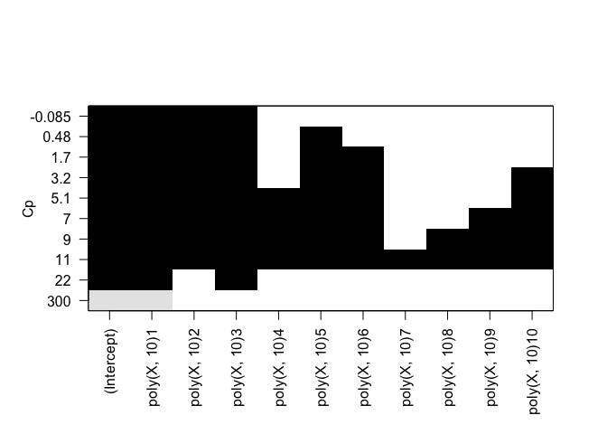
plot(rfit.full, scale="Cp")

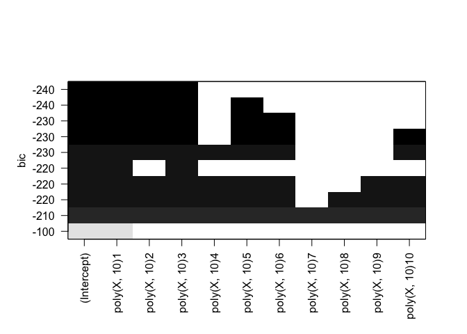
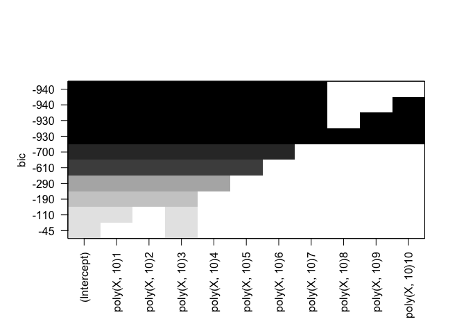
plot(rfit.full, scale="bic")

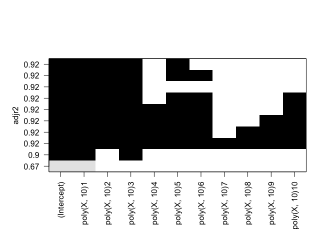
plot(rfit.full, scale="adjr2")

Cp: B0, B1, B2, B3, B8 BIC: B0, B1, B2, B3 Adjusted R^2: B0, B1, B2, B3, B8

rfit.full = regsubsets(Y ~ poly(X, 10), data=df, nvmax=10, method="forward")
plot(rfit.full, scale="Cp")

plot(rfit.full, scale="bic")

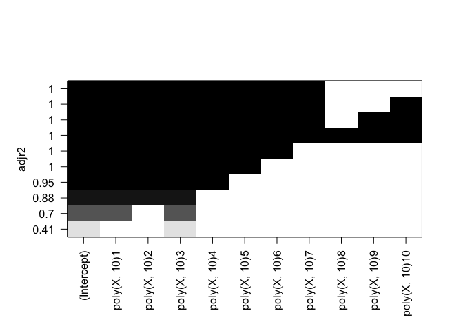
plot(rfit.full, scale="adjr2")

rfit.full = regsubsets(Y ~ poly(X, 10), data=df, nvmax=10, method="backward")
plot(rfit.full, scale="Cp")

plot(rfit.full, scale="bic")

plot(rfit.full, scale="adjr2")

Identical results for both forward and backward stepwise selection.

library(glmnet)

## Loading required package: Matrix

## Loading required package: foreach

## Loaded glmnet 2.0-10

set.seed(1)

x.lasso = model.matrix(Y ~ poly(X, 10), data=df)[, -1]
y.lasso = Y

lasso.cv = cv.glmnet(x.lasso, y.lasso, alpha=1)
plot(lasso.cv)

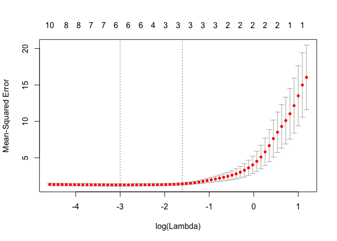
bestlam = lasso.cv$lambda.min
lasso = glmnet(x.lasso, y.lasso, alpha=1, lambda=bestlam)
lasso.coef = predict(lasso, type="coefficients")
lasso.coef

## 11 x 1 sparse Matrix of class "dgCMatrix"
##                       s0
## (Intercept)    1.2516849
## poly(X, 10)1  32.2328511
## poly(X, 10)2   5.0281917
## poly(X, 10)3  18.4941991
## poly(X, 10)4   .        
## poly(X, 10)5  -0.8580825
## poly(X, 10)6   0.5029473
## poly(X, 10)7   .        
## poly(X, 10)8   .        
## poly(X, 10)9   .        
## poly(X, 10)10 -0.3194101

Non zero coefficient estimates for B0, B1, B2, B3, B8. Identical results as obtained by subset/stepwise methods using Cp or AdjR2 metrics.

b7 = 1
Y = b0 + b7*X^7 + eps
df = data.frame(Y=Y, X=X)

rfit.full = regsubsets(Y ~ poly(X, 10), data=df, nvmax=10)
plot(rfit.full, scale="Cp")

plot(rfit.full, scale="bic")

plot(rfit.full, scale="adjr2")

Cp: All but B9, B10 BIC: All but B8, B9, B10 Adjusted R^2: All but B9, B10

x.lasso = model.matrix(Y ~ poly(X, 10), data=df)[, -1]
y.lasso = Y

lasso.cv = cv.glmnet(x.lasso, y.lasso, alpha=1)
lasso = glmnet(x.lasso, y.lasso, alpha=1)
lasso.coef = predict(lasso, type="coefficients", s=lasso.cv$lambda.min)
lasso.coef

## 11 x 1 sparse Matrix of class "dgCMatrix"
##                        1
## (Intercept)    -19.67344
## poly(X, 10)1   742.76455
## poly(X, 10)2  -586.83476
## poly(X, 10)3   911.82687
## poly(X, 10)4  -376.52253
## poly(X, 10)5   279.41009
## poly(X, 10)6   -27.87789
## poly(X, 10)7    16.46163
## poly(X, 10)8     .      
## poly(X, 10)9     .      
## poly(X, 10)10    .

All Beta polynomials up to 5th power. All variable selection methods are failing quite badly here.